Spectrum Extraction Quickstart

Specreduce provides a flexible toolset for extracting a 1D spectrum from a 2D spectral image, including steps for determining the trace of a spectrum, background subtraction, extraction, and wavelength calibration.

This quickstart covers the basic spectrum extraction and calibration steps for a synthetic science spectrum accompanied by He and Ne arc-lamp spectra for wavelength calibration.

This tutorial is written as a Jupyter Notebook. You can run it by copying it (and the quickstart.py module) from GitHub, or from your own specreduce installation under the docs/getting_started directory.

import warnings
import numpy as np
import matplotlib.pyplot as plt
import astropy.units as u

from astropy.modeling import models

from specreduce.tracing import FitTrace
from specreduce.background import Background
from specreduce.extract import BoxcarExtract, HorneExtract
from specreduce.wavecal1d import WavelengthCalibration1D

from quickstart import make_science_and_arcs, plot_2d_spectrum

plt.rcParams['figure.constrained_layout.use'] = True

Data preparation

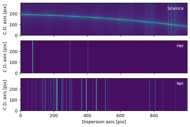
First, we read in our science and arc spectra. We use synthetic data created by the quickstart.make_science_and_arcs utility function, which itself calls specreduce.utils.synth_data.make_2d_arc_image and specreduce.utils.synth_data.make_2d_spec_image. The science frame (sci) and the two arc frames (arc_he and arc_ne) are returned as astropy.nddata.CCDData objects with astropy.nddata.StdDevUncertainty uncertainties.

sci2d, (arc2d_he, arc2d_ne) = make_science_and_arcs(1000, 300)

fig, axs = plt.subplots(3, 1, figsize=(6, 4), sharex='all')
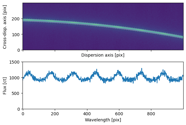
plot_2d_spectrum(sci2d, ax=axs[0], label='Science')
for i, (arc, label) in enumerate(zip((arc2d_he, arc2d_ne), "HeI NeI".split())):
    plot_2d_spectrum(arc, ax=axs[i+1], label=label)
plt.setp(axs[:-1], xlabel='')
plt.setp(axs, ylabel='C.D. axis [pix]');

Spectrum Tracing

The specreduce.tracing module provides classes for calculating the trace of a spectrum on a 2D image. Traces can be determined semi-automatically or manually and are used as inputs for the remaining extraction steps. Supported trace types include:

• specreduce.tracing.ArrayTrace

• specreduce.tracing.FlatTrace

• specreduce.tracing.FitTrace

Each trace class takes the 2D spectral image as input, along with any additional information needed to define or determine the trace (see the API docs for required parameters).

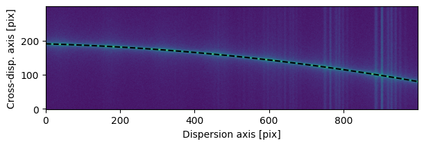
In this example, the spectrum exhibits significant curvature along the cross-dispersion axis, so FlatTrace is not suitable. Instead, we use FitTrace, which fits an Astropy model to the trace.

We choose to fit a third-degree polynomial and bin the spectrum into 40 bins along the dispersion axis. FitTrace estimates the PSF centroid along the cross-dispersion axis for each bin, and then fits the model to those centroids. Binning along the dispersion axis helps stabilize the fit against noise if the spectrum is faint.

trace = FitTrace(sci2d, bins=40, guess=200, trace_model=models.Polynomial1D(3))

fig, ax = plot_2d_spectrum(sci2d)
ax.plot(trace.trace, 'k', ls='--');

Background Subtraction

The specreduce.background module contains tools to generate and subtract a background image from the input 2D spectral image. The specreduce.background.Background object is defined by one or more windows, and can be generated with:

• specreduce.background.Background.one_sided

• specreduce.background.Background.two_sided

The center of the window can either be passed as a float, integer, or trace

bg = Background.one_sided(sci, trace, separation=5, width=2)

or, equivalently

bg = Background.one_sided(sci, 15, separation=5, width=2)

The estimated background image can be accessed via specreduce.background.Background.bkg_image and the background-subtracted image via specreduce.background.Background.sub_image.

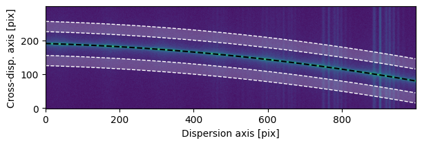
Let’s calculate and remove a two-sided background estimate.

background = Background.two_sided(sci2d, trace, separation=50, width=30)

fig, ax = plot_2d_spectrum(sci2d)
ax.plot(trace.trace, 'k--')
for bkt in background.traces:
    ax.fill_between(np.arange(sci2d.shape[1]),
                    bkt.trace - background.width / 2,
                    bkt.trace + background.width / 2,
                    fc='w', alpha=0.2)
    ax.plot(bkt.trace+background.width/2, 'w--', lw=1)
    ax.plot(bkt.trace-background.width/2, 'w--', lw=1)

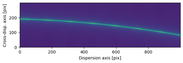
sci2d_clean = background.sub_image()

fig, ax = plot_2d_spectrum(sci2d_clean.flux.value)

Spectrum Extraction

The specreduce.extract module extracts a 1D spectrum from an input 2D spectrum (likely a background-extracted spectrum from the previous step) and a defined window, using one of the following implemented methods:

• specreduce.extract.BoxcarExtract

• specreduce.extract.HorneExtract

The methods take the input image and trace as inputs, an optional mask treatment agrumtn, and a set of method-specific arguments fine-tuning the behavior of each method.

Boxcar Extraction

Boxcar extraction requires a 2D spectrum, a trace, and the extraction aperture width.

aperture_width = 20
e = BoxcarExtract(sci2d_clean, trace, width=aperture_width)
sci1d_boxcar = e.spectrum

The extracted spectrum can be accessed via the spectrum property or by calling the extract object, which also allows you to override the values the object was initialized with.

fig, axs = plt.subplots(2, 1, figsize=(6, 4), sharex='all')
plot_2d_spectrum(sci2d_clean.flux.value, ax=axs[0])
axs[0].fill_between(np.arange(sci2d_clean.shape[1]),
                    trace.trace - aperture_width / 2,
                    trace.trace + aperture_width / 2,
                    fc='w', alpha=0.25, ec='k', ls='--')

axs[1].plot(sci1d_boxcar.flux)
plt.setp(axs[1],
         ylim = (0, 1500),
         xlabel=f'Wavelength [{sci1d_boxcar.spectral_axis.unit}]',
         ylabel=f'Flux [{sci1d_boxcar.flux.unit}]');
fig.align_ylabels()

Horne Extraction

Horne extraction (a.k.a. optimal extraction) fits the source’s spatial profile across the cross-dispersion direction using one of two approaches:

• A Gaussian profile (default). Optionally, you may include a background model (default is a 2D polynomial) to account for residual background in the spatial profile. This background-model option is not supported with the interpolated profile.

• An empirical interpolated profile, enabled via interpolated_profile.

Using the interpolated_profile option:

• The image is binned along the wavelength axis (number of bins set by n_bins_interpolated_profile), averaged within each bin, and then interpolated (linear by default; the interpolation degree in x and y can be set via interp_degree_interpolated_profile) to form an empirical spatial profile.

• You can select this mode by passing a string to use default settings, or a dictionary to override the defaults.

Examples: Use the interpolated profile with default bins and interpolation degree:

interp_profile_extraction = extract(spatial_profile='interpolated_profile')

Use 20 bins instead of the default of 10:

interp_profile_extraction = extract(spatial_profile={
    'name': 'interpolated_profile',
    'n_bins_interpolated_profile': 20
})

Use cubic interpolation instead of the default linear:

interp_profile_extraction = extract(spatial_profile={
    'name': 'interpolated_profile',
    'interp_degree_interpolated_profile': 3
})

The Horne extraction algorithm requires a variance array. If the input image is an astropy.nddata.NDData object with image.uncertainty provided, that uncertainty will be used. Otherwise, you must supply the variance parameter.

extract = HorneExtract(image - bg, trace, variance=var_array)

As usual, parameters can be set when creating the HorneExtract object or overridden when calling the object’s extraction method.

e = HorneExtract(sci2d_clean, trace)
sci1d_horne = e.spectrum

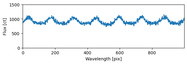
fig, ax = plt.subplots(1, 1, figsize=(6, 2), sharex='all')
ax.plot(sci1d_horne.flux)
plt.setp(ax,
         ylim = (0, 1500),
         xlabel=f'Wavelength [{sci1d_horne.spectral_axis.unit}]',
         ylabel=f'Flux [{sci1d_horne.flux.unit}]')
ax.autoscale(axis='x', tight=True)

Wavelength Calibration

The specreduce.wavecal1d.WavelengthCalibration1D class provides tools for one-dimensional wavelength calibration given a number of arc calibration spectra and corresponding catalog line lists.

First, we need to extract the arc spectra from the 2D arc frames using the trace we calculated from our science spectrum. Next, we instantiate a WavelengthCalibration1D object and pass the arc spectra and the line lists to use. We also pass it the wavelength unit we want to use, the line list bounds (we know that our instrument setup gives a spectrum that covers approximately the range of 500-1000 nm), and the number of strongest lines to include from the catalog line lists.

arc1d_he = BoxcarExtract(arc2d_he, trace, width=aperture_width).spectrum
arc1d_ne = BoxcarExtract(arc2d_ne, trace, width=aperture_width).spectrum

wc = WavelengthCalibration1D([arc1d_he, arc1d_ne],
                             line_lists=["HeI", "NeI"],
                             line_list_bounds=(500, 1000),
                             n_strogest_lines=15,
                             unit=u.nm)

Line Finding

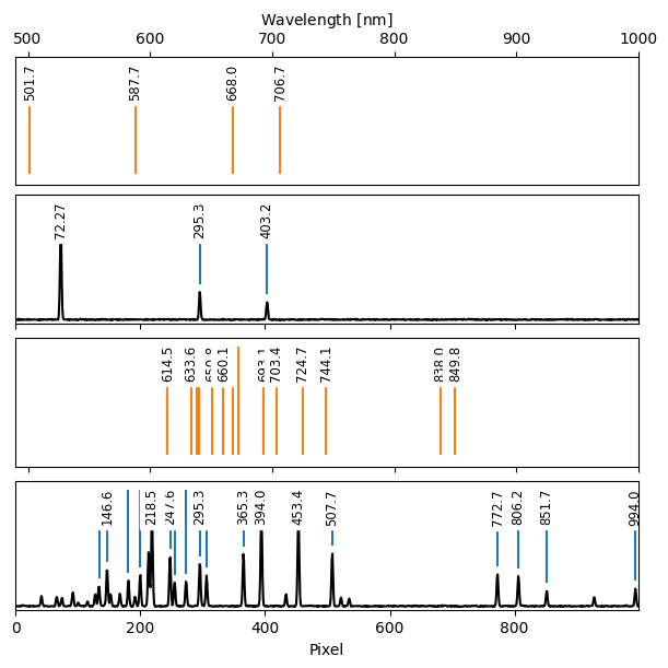
Next, we wse WavelengthCalibration1D.find_lines to detect emission lines in the arc spectra. Then, we visualize the catalog lines alongside the arc spectra and the detected lines with WavelengthCalibration1D.plot_fit.

with warnings.catch_warnings():
    warnings.simplefilter('ignore')
    wc.find_lines(3, noise_factor=25)

fig = wc.plot_fit(figsize=(6, 6))
plt.setp(fig.axes[::2], xlim=(490, 1000));

Wavelength Solution Fitting

With the observed and catalog lines identified, we can now compute the wavelength solution, represented by a specreduce.wavesol1d.WavelengthSolution1D object. The wavelength calibration class provides several methods; here we use the interactive fit_lines method. This method:

• takes a list of matched pixel positions and their corresponding wavelengths,

• fits a polynomial to these pairs, and

• refines the solution by incorporating all observed and catalog lines within a specified pixel distance of the initial fit.

ws = wc.fit_lines([72, 295, 403, 772], [588, 668, 707, 838],
                  degree=3, refine_max_distance=5)

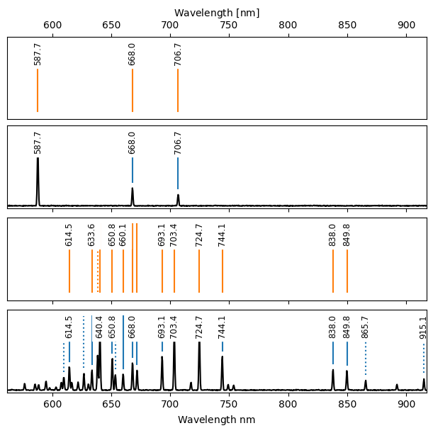
Now we can visualize the observed and catalog lines again. Set obs_to_wav=True to display the observed arc spectra and lines in wavelength space. Matched fitted observed and catalog lines are shown with solid lines; unmatched lines are shown with dashed lines.

fig = wc.plot_fit(figsize=(6, 6), obs_to_wav=True)
plt.setp(fig.axes, xlim=ws.p2w([0, 1000]));

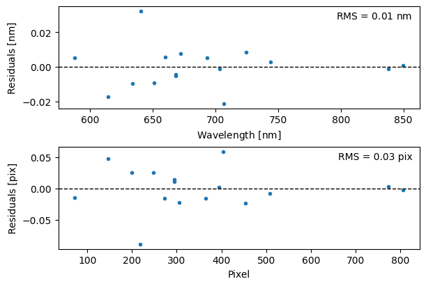
We can also visualize the residuals between the observed and catalog lines (either in wavelength or pixel space) to assess the quality of the fit.

fig, axs = plt.subplots(2, 1, figsize=(6, 4), constrained_layout=True)
wc.plot_residuals(ax=axs[0], space="wavelength")
wc.plot_residuals(ax=axs[1], space="pixel")
fig.align_ylabels()

Spectrum Resampling

With a satisfactory wavelength solution in hand, we can finalize the reduction. You have two options:

• Attach the gwcs object from the WavelengthSolution1D to the science spectrum, or

• Resample the science spectrum onto a defined wavelength grid using WavelengthSolution1D.resample.

Here, we choose to resample the spectrum.

sci1d_resampled = ws.resample(sci1d_boxcar)

fig, ax = plt.subplots(figsize=(6, 3))
ax.plot(sci1d_resampled.spectral_axis, sci1d_resampled.flux)
plt.setp(ax,
         ylim = (0, 1500),
         xlabel=f"Wavelength [{sci1d_resampled.spectral_axis.unit}]",
         ylabel=f"Flux density [{sci1d_resampled.flux.unit}]")
ax.autoscale(axis='x', tight=True)

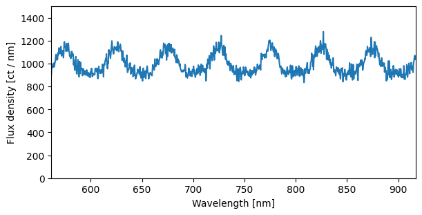
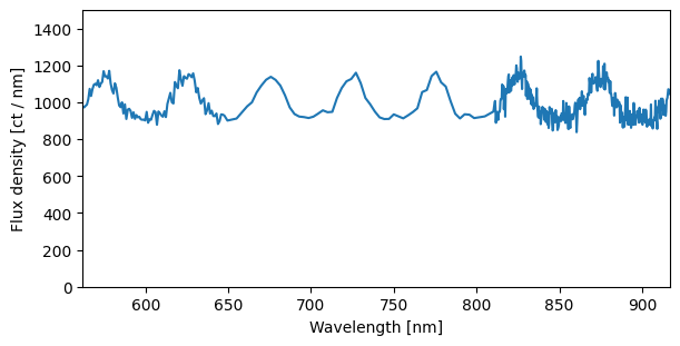
By default, the resample method creates a linear wavelength grid spanning the spectrum’s range, with as many bins as there are input pixels. However, you can also fully customize the grid by supplying explicit bin_edges.

bin_edges = np.concatenate([np.geomspace(ws.pix_to_wav(0), 650, num=100),
                            np.linspace(660, 800, 50),
                            np.linspace(810, ws.pix_to_wav(999), 400)])

sci1d_resampled = ws.resample(sci1d_boxcar, bin_edges=bin_edges)

fig, ax = plt.subplots(figsize=(6, 3))
ax.plot(sci1d_resampled.spectral_axis, sci1d_resampled.flux, '-')
plt.setp(ax,
         ylim = (0, 1500),
         xlabel=f"Wavelength [{sci1d_resampled.spectral_axis.unit}]",
         ylabel=f"Flux density [{sci1d_resampled.flux.unit}]")
ax.autoscale(axis='x', tight=True)

Finally, we can save the spectrum as fits.

sci1d_resampled.write('science_spectrum.fits', overwrite=True)